🦖
Generating Fantasy Maps With Statistical Mechanics 🧙♂️🗺️
An unusual application of the 2D Ising model
#statistical-physics
#generative-programming
#maps-generation
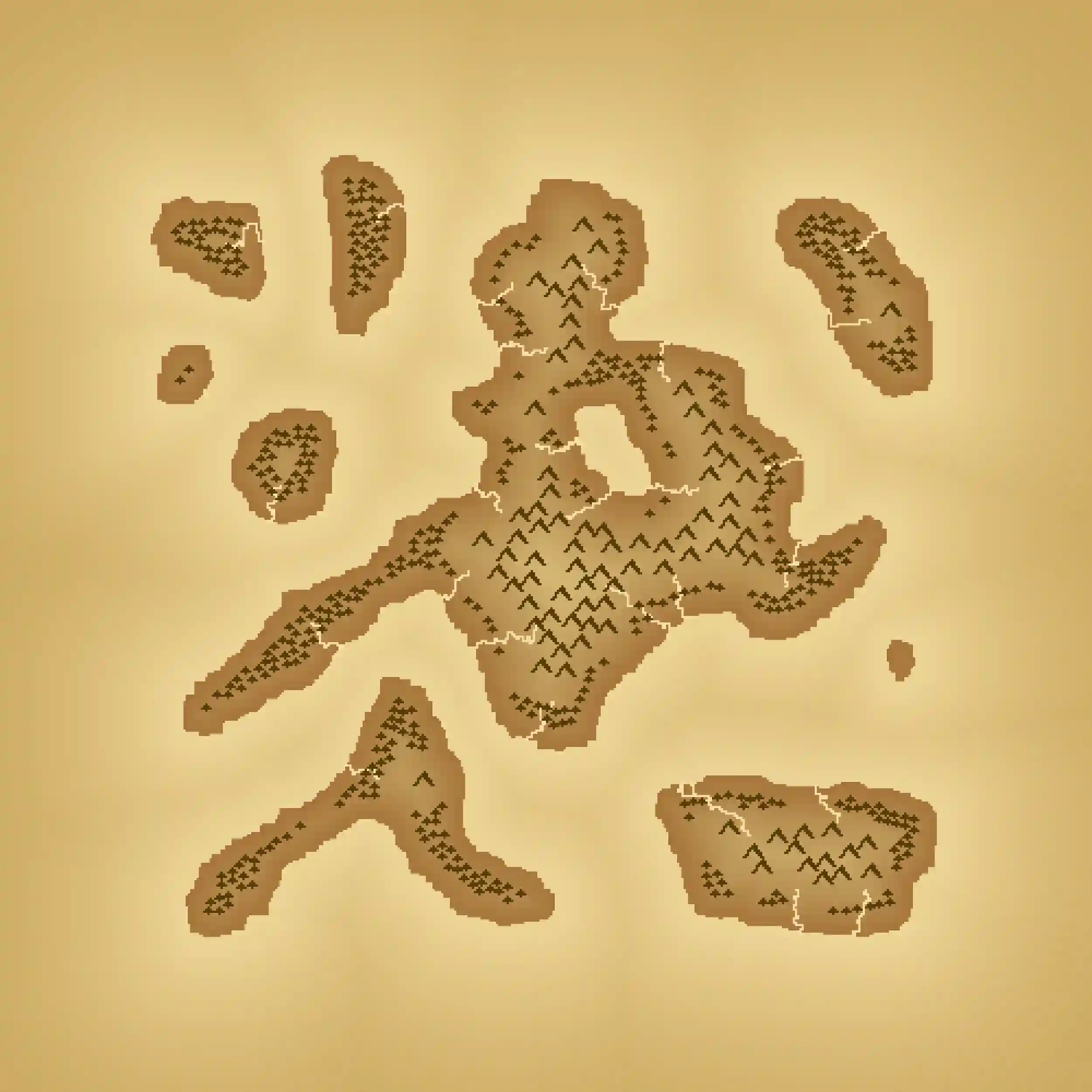
A map generated following the scheme presented in this post.
Introduction
I was looking at some cool blog posts on generative programming and, in particular, on how to programmatically generate maps. In particular, I was looking at the approach proposed in 1, and the one reported in 2 3. In this post, I will describe an alternative way of generating sea/terrain patterns, using a model from Statistical Physics, that should resemble a world map.
The procedure that will be described is inefficient with respect to other algorithms. However,I think that the intriguing aspect lies in the application of a model from the field of Statistical Physics to a task entirely unrelated to its conventional domain.
A C++ implementation of the procedure presented in this post is available here .
The 2D Ising Model
The Ising model was introduced in Statistical Physics to understand phase transitions in ferromagnetic materials. Despite its simplicity, this model plays a central role in the understanding of phase transitions 4. The model describes a system of particles having fixed positions and forming a grid where their only degree of freedom is represented by their spin orientation (either up or down).
The model takes its name from Ernst Ising, which was the first to demonstrate that in one dimension, this system does not undergo any phase transition. However, when we go from 1D to 2D, things start to get more interesting.
In fact, in two dimensions, there exists a temperature called critical, $T_C$, for which the system undergoes a phase transition (between the paramagnetic and ferromagnetic phase). When the system is at higher temperatures with respect to the critical one, the system does not show any correlation. However, when the temperature reaches the critical temperature, the system exhibits correlations at all scales. Finally, in a low-temperature regime, the system will be dominated by either up or down spin.
The system is described by the following Hamiltonian5: $$ \mathcal{H}= -\sum_{\langle ij \rangle} J_{ij} s_{i}s_{j} + \mu\sum_i h_i s_i $$ where $s_i$ and $s_j$ can be equal to either $\uparrow$(+1) or $\downarrow$(-1), $J_{ij}$ is the coupling constant which we can assume equal for all spin-spin couple (i.e. $J_{ij}\equiv J$), $\mu$ is the magnetic moment and $h_i$ is the external magnetic field acting on site $i$. In this post we will be consider the case where no external magnetic fields are applied (i.e. $h_i=0\ \ \forall i$).
It's worth emphasizing that the system is regarded as being connected to a heat bath that induces stochastic spin flips.
We can see how the system behave in three different temperature regimes by running a Monte Carlo simuluation using the Metropolis-Hasting algorithm6 7:
Low Temperature Regime $T$ << $T_C$
Critical Temperature Regime $T$ $\approx$ $T_C$
High Temperature Regime $T$ >> $T_C$
To build confidence in the model and to see the effect of the temperature and coupling constant, you can experiment and become familiar with its characteristics by playing around with the interactive widget below. You should notice something happen when $T/J\approx 2.269$.
Temperature, T
Coupling Constant, J
Generating Sea/Terrain areas
So, how can we exploit this in order to generate sea/land patterns?
The idea is to allocate land to the pixels with spin $\uparrow$ and sea to spin $\downarrow$.
By starting with the lattice in a random configuration and slowly reducing its temperature below the critical one from one Monte Carlo iteration to another, we should be able to move our system to a state where the spatial correlation resembles the sea-land distribution in a world map. Since we want to have a map centered around the continents (i.e., the land areas), we wish to avoid terrain that touches our lattice boundaries. In order to do so, we can constrain all the lattice sites near the boundaries to be in the spin $\downarrow$ state.
From the simulation above, we can notice two main things:
- The generated map is “blocky” due to the relatively small number of spin sites. In order to achieve maps with higher resolution, we have to increase the number of sites. However, this will increase the computational time required to generate the map since we will need more iterations to reach a state that could serve as a map.
- When we reach a spin distribution that could resemble sea/terrain area, some “noisy” pixel remains. In such a small lattice (60$\times$60), we may think of them as tiny islands or lakes; however, when we are interested in higher resolution maps, these pixels behave like actual noise.
As for the first point, there are limited options for intervention. However, regarding the second point, there is a viable solution. In fact, we can remove “noisy” pixels by “freezing out” our system.
What does this mean?
We can simply run some more Monte Carlo iteration by setting our system temperature to 0. In this way, only favorable energy transition will be accepted. If we think of the situation where a $\uparrow$ is surrounded by $\downarrow$ spins, the only favorable way is to flip the spin of the particle in the middle.
You can try this freezing procedure by running the simulation below and then pressing the freeze button.
We can summarize this first part as follows:
Algorithm : Generating sea/terrain pattern
- Initialize a 2D N$\times$N spin lattice with a random distribution of spin.
- Start the system at a $T>T_C$
- Use the simulated annealing algorithm to slowly lower the system temperature below the critical one.
- Freeze the system by taking some Monte Carlo iteration with $T=0$.
Side note: Dungeons generation
The “freezing” procedure comes in handy also for generating dungeon-like maps instead of world maps. In fact, if we take some iteration of our lattice at a temperature higher than the critical one and then abruptly freeze out our system, we can generate patterns that are similar to a dungeon map rather than a world map.
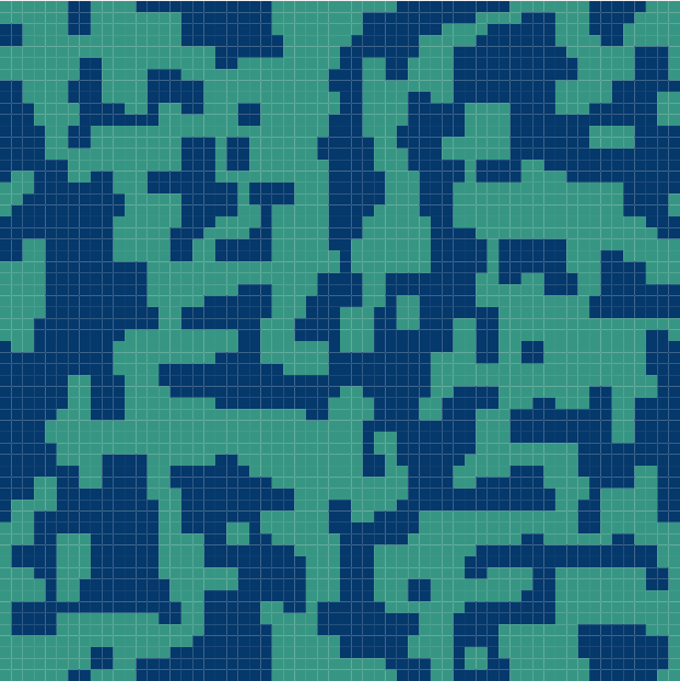
Pattern generated by taking some iteration at $T\approx 2 \ T_C$ prior to set the system temperature to 0.
Creating an Height map
Now that we have a grid with sea/terrain-like areas, we can try to construct a sort of height map, giving our maps a bit of variation and less flat colors.
The first thing that I tried was to associate each lattice site with a height depending on its distance from the closer coastline. For small-size lattices, this can be achieved with a breadth-first search.
However, I have noticed that this algorithm does not scale well with bigger lattices, so I tried another approach based on an image processing technique:
Algorithm : Generating height map
- Apply an edge-detection filter to the generated sea/terrain lattice map in order to extract coastline positions within the lattice.
- Loop over each lattice site and assign as heigth the minimum distance between the cell location and all of the coastline cells, multiplied for the cell spin.
The first step is done by convoluting our lattice with an edge-detection filter, which is a small matrix of the kind:
$$ \omega = \begin{pmatrix} -1 & -1 & -1\\\ -1 & 8 & -1\\\ -1 & -1 & -1 \end{pmatrix} $$ and the convolution operation is given by: $$ I(i,j) = \omega * L = \sum_{x=-a}^{a} \sum_{y=-b}^{b} \omega(x,y) L(i-x,y-j) $$ where $\omega$ is the convolution kernel, $L$ is the original lattice “image”, $I$ is the filtered lattice “image”, $a$ is the kernel row number and $b$ is the kernel column number. At this point the coastline can be extracted as the set of cells with negative values in the filtered lattice.
At this point we can associate to each cell site an height value based on the minimum distance from coastline as follow: $$ \rm{height}(i,j) = \min_{c_{kl}} \sqrt{(i-k)^2+(j-l)^2} $$ where $c_{kl}$ indicates a generic coastline cell located at position $(k,l)$. The map generated with the widget below will interpolate between three colors for the positive height maps and between two colors for the negative ones in order to have a shaded map.
Trees, mountains and rivers 🌳⛰️🏞️
From what we have seen up to now, we’re faced with a wasteland, which is far from visually appealing.
However, we can transform this barren landscape into a more natural and captivating environment by using the height map we’ve just generated. This height map allows us to introduce various natural features, such as trees, mountains, and rivers.
The process of incorporating trees and mountains is relatively straightforward. We can randomly select a set of points, possibly applying certain height-based filters, to determine where these features should be placed. Once we’ve identified these points, we can start the creation of pixel art representations resembling either mountains or trees at each selected location. The key consideration here is ensuring that these pixel art graphics do not overlap, and we can achieve this by keeping a record of the sampled points and excluding those that are too close to one another.
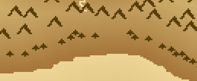
Example of mountains and trees pixel arts used in the generated maps.
Rivers present a greater complexity in their generation compared to the relatively straightforward modeling of trees and mountains.
A basic approach for generating a river using the height map is described below:
Algorithm : Generating a river
- Pick a random cell having a height greater than 0 from the height map and store its position in an array representing the river path.
- Look at the nearest neighbors of the selected cell and put it inside an array of all the cells with a lower height.
- Pick one cell at random between the lower-elevation cells array and append its position to the river path array.
- If the selected cell height is greater than 0, then go to (2) using this cell as a starting point; otherwise, exit from the procedure.
To illustrate the results of this procedure, let’s consider a simplified scenario: a circular island whose height map is defined by a parabolic function.
Example maps 🗺️
Using the set of procedures described above is possible to obtain maps similar to these:
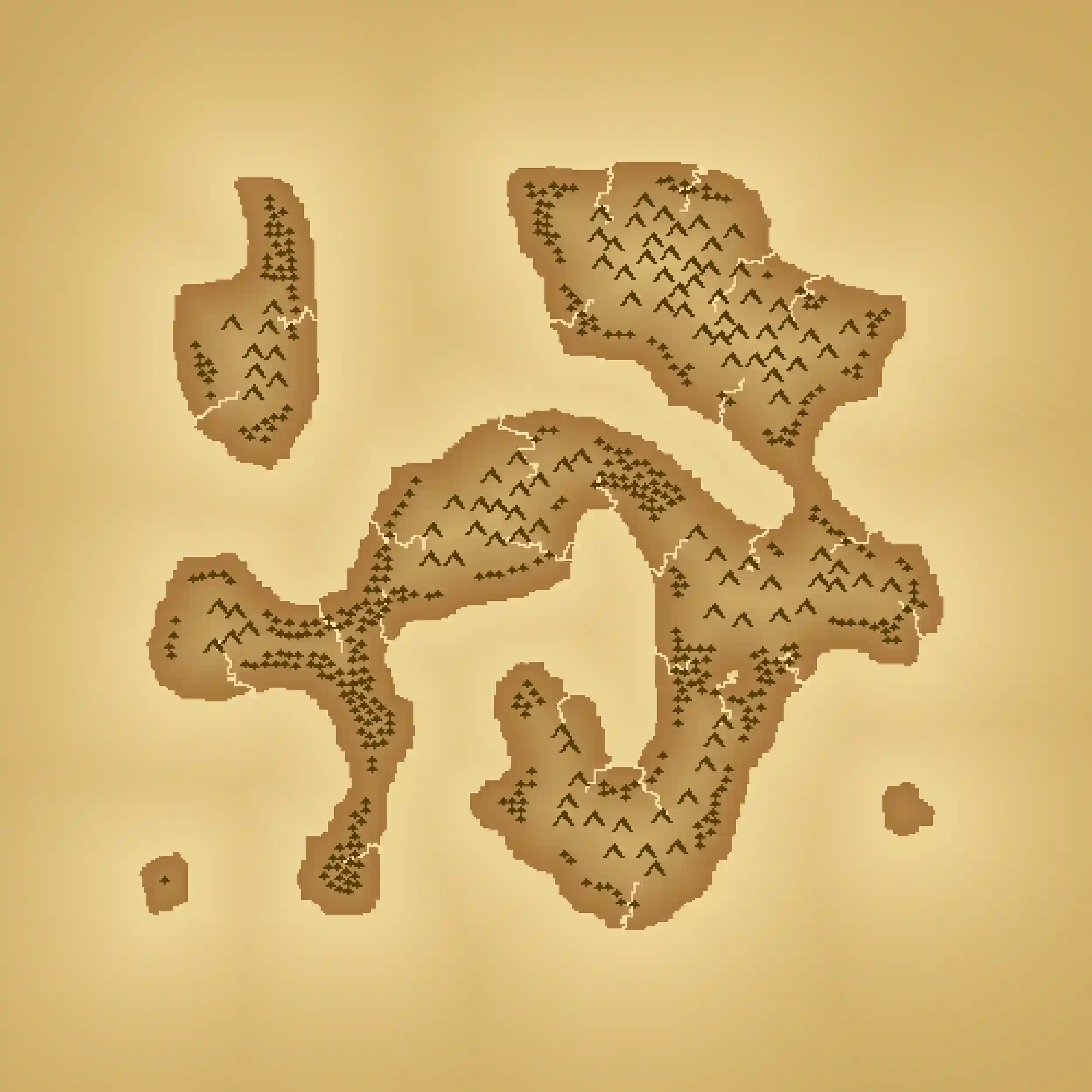
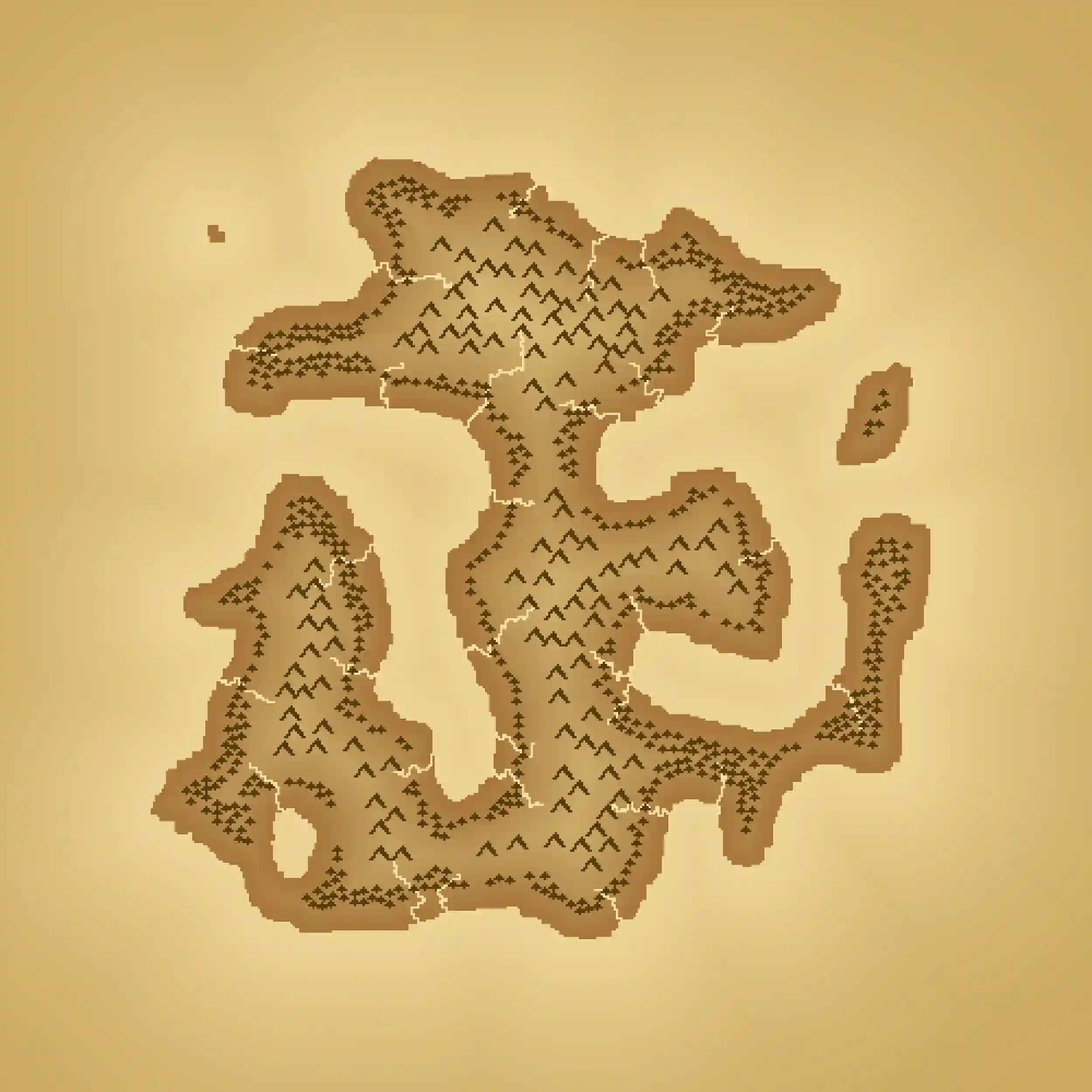
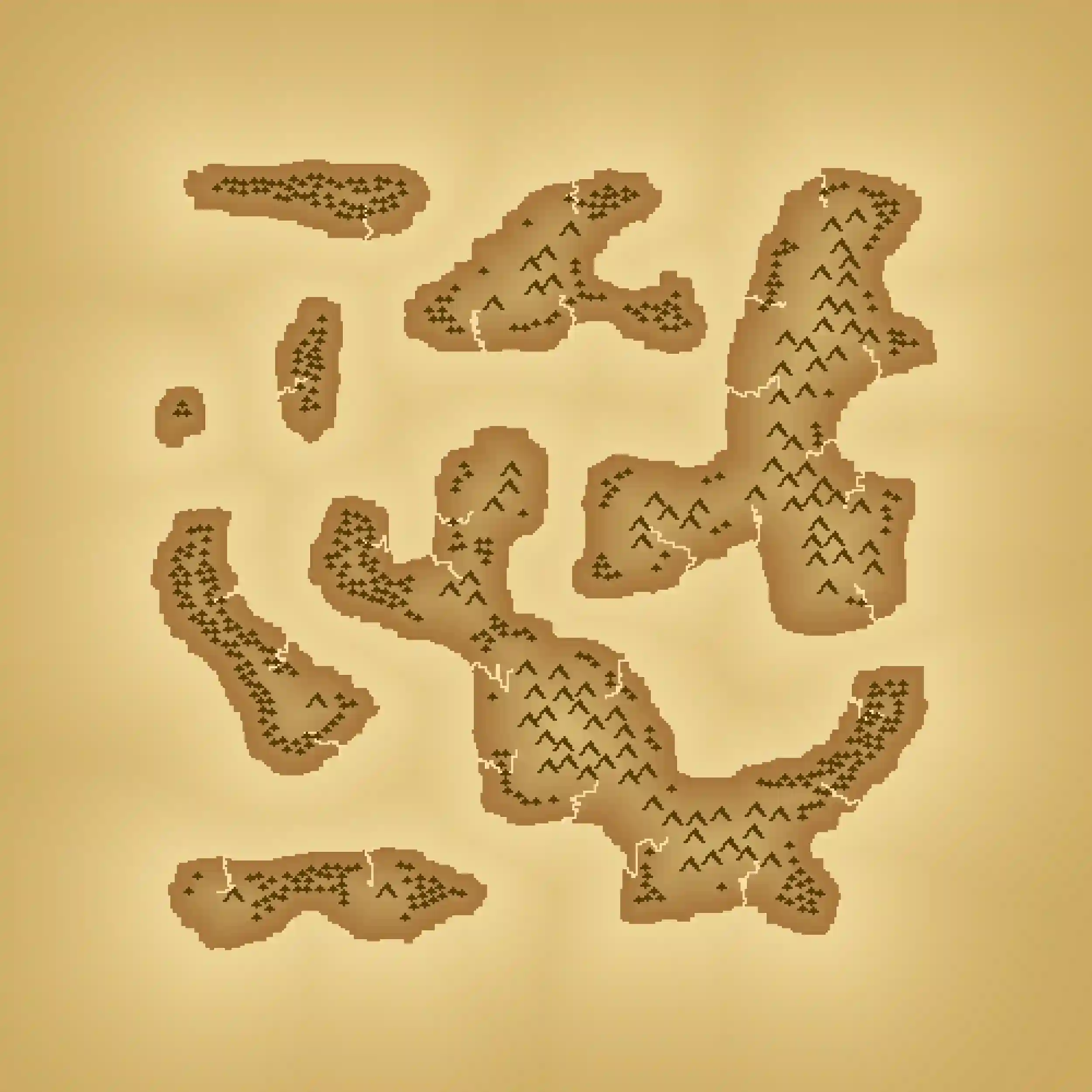
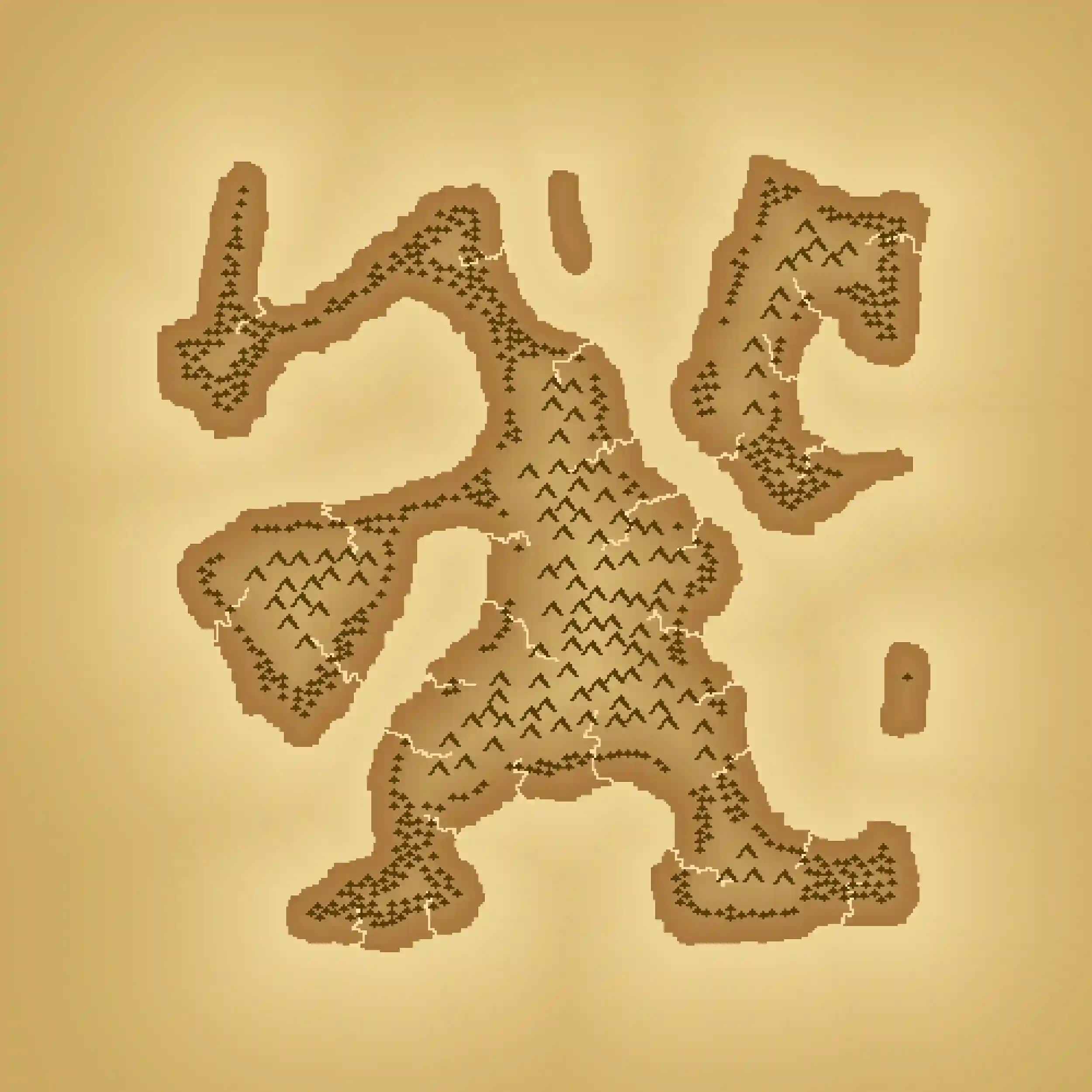
It is possible to obtain different sea/land ratios by playing with the total number of Monte Carlo iterations of the algorithm.
Possible improvements
Finally, I want to add a couple of improvements that could be considered.
First of all, for the maps we generated, we opted to position trees within a specific range of heights, spanning from a minimum to a maximum elevation. We selected to generate mountainous terrain beyond this maximum elevation suitable for tree growth. However, since we have used the distance from the coast as height, trees, and mountains displacement are very similar in all the generated maps. An enhancement to this approach could involve employing a noise function to determine the locations of forests and mountains.
Secondly, an idea for speeding up the map generation is to use a non-square lattice (e.g., triangular lattices, Voronoi cells). In addition to this, it should also be possible to generate smaller lattices and then use noisy edges as proposed in [8] for delimiting terrain regions using vector graphics instead of raster bitmap.
Finally, it would be nice to add cities and roads between them using some procedurally generated names.
If you have any suggestions, please feel free to contact me by sending an email .
Footnotes
-
http://www-cs-students.stanford.edu/~amitp/game-programming/polygon-map-generation/ ↩︎
-
Huang, Kerson. Statistical mechanics. John Wiley & Sons, 2008. ↩︎
-
For the non-physicist reader, the Hamiltonian of a physical system describe its energy. In this case, since the particles are constrained in a well-defined fixed position, and thus we have no kinetic energy term, we can “interpret” this as the energy due to spin-spin interactions. ↩︎
-
https://en.wikipedia.org/wiki/Metropolis%E2%80%93Hastings_algorithm ↩︎